Waveguide Loss Measurement

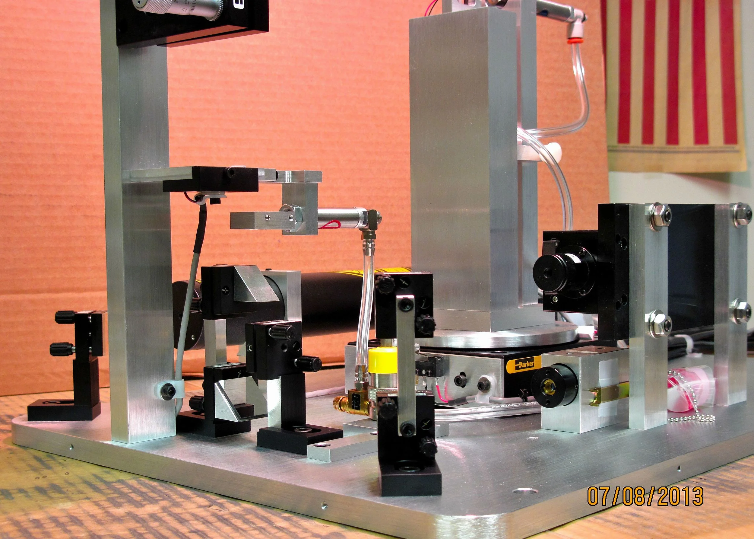
This option measures loss of optical waveguides by scanning a fiber optic probe and photodetector down the length of a propagating streak to measure the light intensity scattered from the surface of the guide. The assumption is that at every point on the propagating streak the light scattered from the surface and picked up by the fiber is proportional to the light which remains within the guide. The best exponential fit to the resulting intensity vs distance curve yields the loss in db/cm. This method offers the advantages of quickness (typical measurement time, including the exponential fit, is 2-3 minutes) and simplicity (absolutely no sample preparation beyond creation of the layers which form the guide is required).

• Comparison to other methods: The optical fiber method is identical in concept to the CCD camera approach for measuring the decay of the propagating streak but the camera must have very uniform response sensitivity over the full array. With the scanning fiber method, only a small single-element silicon or InGaAs detector is used and spatial uniformity is not an issue. In addition, for loss measurements beyond 1100 nm high quality spatially uniform IR cameras are quite expensive.

Various multiple coupling prism approaches have also been used to provide accurate loss results. In the typical two prism technique, one prism is used to couple light into the guide and another prism is moved down the guide to couple out and measure the light remaining within the guide at multiple points. With this technique it is, however, very difficult to ensure that the coupling efficiency into the guide at the first prism is not changed as the second movable prism is brought into and out of contact with the sample. Unless the coupling faces of the prisms lie precisely in the same planes and the samples themselves are extremely flat, mechanical stresses as the second prism is clamped to the sample can cause a change in the coupling efficiency or possibly complete loss of contact at the first prism. To overcome this problem, various three prism approaches have been proposed to compensate for coupling efficiency changes at the first prism. The main problem with these approaches is that the apparatus is mechanically quite complex and measurements are slow because of the need to couple and decouple the sample to the movable prism multiple times while monitoring that the coupling efficiency of the first prism does not change.

Another technique involves using a single prism to couple light into a sample and then immersing the sample into a bath filled with index matching fluid to couple out the light remaining within the guide. This technique is limited to relatively low index guides since the fluid must be closely matched to the index of the guide and the maximum index available for matching fluids is limited. Higher index fluids, moreover, are costly and often caustic or even poisonous, and use of a variety of different fluids may be required if working with waveguides over a range of indices. In addition, waveguide materials, especially polymers, may react either obviously or more subtly when placed in contact with the matching fluids, leading to loss behavior anomalies. A final requirement is that the sample must usually be cut or broken into a long narrow piece because of bath size/shape limitations. Cutting or breaking samples invariably generates large numbers of particles which can settle onto the sample surface and, unless extreme care is taken, it is difficult to avoid some scratching of the sample surface. While normal measurements of index and thickness are relatively tolerant of surface scratches or small particles, surface scattering losses, which often dominate the loss behavior, are extremely sensitive to the introduction of particles and scratches.

The scanning fiber method offers the advantages of mechanical and operational simplicity, speed, elimination of costly or toxic index matching fluids, and absolutely no sample preparation, but samples must exhibit some surface scattering loss to provide a means of sampling the light intensity within the guide. In our experience, this is rarely a significant limitation since even low loss waveguides (below a few tenths of a db/cm) usually provide more than enough scattered light to be measurable. A more important requirement, is that the scattering behavior of the sample surface be uniform for the propagation path over which loss is measured. If, for example, one part of the streak scatters more than another, the scattered light at each point is not an accurate representation of the light remaining within the guide and the resulting intensity vs distance curve may not shown an exponential shape. While the 2010/M system displays the optimum fitted exponential superimposed on the raw intensity vs distance curve (see sample measurements below), and it is easy for the user to recognize if the pattern deviates from exponential behavior, accuracy of the loss measurement is reduced when samples exhibit non-exponential patterns. However, since surface scattering is an important mechanism of waveguide loss (and very often the dominant mechanism) if scattering efficiency changes spatially over the surface of the sample, this really means that the loss itself (however it is measured) is changing spatially over the surface of the sample and there is no one single loss figure which is representative of the entire sample. So the presence of a non-exponential curve is an important piece of information in itself, alerting the user that the loss behavior itself is spatially dependent.

• Loss measurement range: The 2010/M’s loss measurement option works over the range from 15 db/cm to ≈ 0.1 db/cm (see sample measurements below). Minimum loss measurable depends on how much light is scattered from the guide and whether the loss profile exhibits significant non-exponential behavior due to spatial variation in the surface scattering efficiency (see discussion above). The best method of ensuring that the loss measurement option provides good characterization for a particular class of guides is to submit samples to Metricon for evaluation.
• Waveguide index range measurable: The option can be used over the full index range measurable with the 2010/M system (1.0 to 3.35, with appropriate prism).
• Repeatability: For guides which exhibit essentially exponential behavior, measurements taken at various points on the sample are usually repeatable to ± 5% (i.e., a 1 db/cm measurement will vary by ± 0.05 db/cm). For guides with significantly non-exponential decay, measurement of individual propagation paths are usually repeatable to ± 5% or less (i.e., a 1 db/cm measurement will vary by ± 0.05 db/cm) but results may vary by ± 20% depending on the exact path which the streak traces down the sample.
• Accuracy: The science of loss measurement is in its infancy and no standards are available which permit certification of absolute loss accuracy. However, observance of an essentially exponential loss decay profile is good evidence that the sample is conforming to theory and the loss measurement apparatus is measuring the decay profile accurately. In the absence of a universally accepted loss accuracy standards, we invite and encourage comparative measurements between our apparatus and other techniques.
• Wavelength measuring range: From 405 to 1064 nm with silicon detector (option 2010/M-WGL1) or 520 to 1600 nm with InGaAs detector (option 2010/M-WGL2).
• Sample size: While measurements can often be made for propagation distances of 25-30 mm from the coupling point, propagation distances of 40-50 mm are desirable, especially for low loss guides. Any sample shape can be accommodated (circular, square, long and narrow). The length of the profiling scan is user adjustable with a maximum scan length of 55 mm. The fiber position is driven by a linear stepper motor with a linear resolution of 20 steps/mm, resulting in typical intensity patterns of 200 to 1000 data points.
• Measurement procedure: The rotary table is first positioned so that the desired mode is excited and a propagating streak is obtained (this is easily done even if the beam is invisible). The fiber is then driven by a stepper motor into close proximity to the prism (at the start of the streak). The fiber is then automatically scanned down the propagation path and the intensity vs distance profile is displayed on the PC monitor. With a mouse, the user then selects the parts of the pattern to be used in the loss calculation, avoiding obvious peaks caused by scratches, particles, or other surface imperfections. Loss in db/cm is then calculated automatically by a least squares fit to the intensity data and the resulting exponential fit is superimposed over the intensity profile. To improve the fit, the portion of the intensity pattern included in the calculation can then be refined or changed and the loss recalculated. At any point, loss intensity patterns and results can be saved to disk or printed out on the system printer. The entire process, from locating the mode to the final loss calculation, requires approximately 2-3 minutes.