CHARACTERIZATION OF OPTICAL WAVEGUIDES/WAVEGUIDE LOSS

With Metricon’s Model 2010/M, waveguide characterization data which typically requires a skilled professional an hour or more to collect with homemade apparatus can now be obtained in 30 seconds or less in a format providing complete documentation of results and measurement conditions.  Thickness and index of the guiding layer (and very often the cladding layer) are easily measured for planar layers, as are the number of modes and effective mode indices and options 2010-WGL1 and 2010-WGL2 permit measurement of waveguide loss. 

Moreover, the mode pattern (plot of reflected intensity vs angle of incidence) can provide the user with a wealth of insight into waveguide behavior which is not available with other thin film measurement methods such ellipsometry or spectrophometry.

CHARACTERIZATION OF GUIDING LAYER THICKNESS AND INDEX, 
CLADDING LAYER, NUMBER OF MODES AND MODE INDICES

For all types of planar guides, the Model 2010/M provides rapid measurement of mode indices, and for step index guides, calculation of guide thickness and refractive index and, in most cases, substrate or cladding index.  In addition, with the standard TE-mode measurement, indices for both guides and substrate materials are measurable along any in-plane direction, while the TM option provides measurement in the perpendicular-plane direction.  

For graded index guides, an index vs depth calculation based on the method of Chiang (J. Lightwave Technology, LT-3, p. 385, April 1985) is provided (see sample lithium niobate waveguide calculation below).  A mode modeling feature is also provided which permits calculation of mode angles and effective indices from single and dual film thickness and index values input by the user.

Until recently, waveguide characterization with the 2010/M has been limited to planar waveguides, but two recent papers (B. Chen et al, IEEE Phot. J., 4(5), 1553-1559 (October 2012) and K. S. Chiang et al, Opt. Engr., 47(3), 034601-1 to 034601-4 (March 2008)) have shown the feasibility of using the 2010/M to measure effective mode indices for arrays of stripe and channel waveguides. 

Major components of the Model 2010/M include: a coupling mechanism which brings the waveguide and the prism into intimate contact in a gentle and reproducible fashion; a laser and a step motor-driven rotary table to vary the angle of incidence of the beam on the prism; and a PC-based controller which employs pattern recognition software to determine effective mode indices (and resulting thickness and index) from the pattern of beam intensity reflected from the base of the prism vs. incident angle.   All aspects of system operation, including table positioning and detection of modes, can be performed fully automatically or manually by the user.  

Further features of interest for integrated optics work include:

Operating wavelength:  Although the standard system operates at 633 nm, most systems for integrated optics provide one or two additional beamlines so that multiple lasers can be used with the system.  The Model 2010/M can be supplied with additional lasers in the 400-1600 nm range, or the system can be configured with a port for a user-supplied laser external to the system.  For such multiple beamline systems, wavelength selection consists simply of opening and closing the appropriate mechanical beam blocks and changeover between wavelengths requires 10 seconds or less.  Popular wavelengths for optical waveguide measurements include 830, 1310 and 1550 nm.  In addition, we have configured systems with 405, 450, 473, 520, 532, 650, 780, 850, 980, and 1064 nm lasers.  
 
Resolution/accuracy:  A high resolution rotary table with software selectable angular resolution of 0.9 or 0.45 minutes is usually ordered as a no-cost option for waveguiding applications.  For this table, effective index (β-value) resolution is .0002 (±.0001) with 0.9 minute operation and .0001 (±.00005), with 0.45 minute operation.  Absolute accuracy of prism coupler measurements are often limited to the ±.0003 range by uncertainties in the measuring prism angle and index.  For many applications, calibration standards are available which will permit absolute index accuracy comparable to the rotary table effective index resolution (±.00005).
 
Coupling arrangement:  The 2010/M's coupling apparatus provides effective and reliable coupling for a broad variety of substrate sizes and thicknesses, permitting attainment of optimum coupling conditions in just a few seconds.  Accurate and reproducible coupling pressure without sample rotation or prism damage is obtained with a
pneumatic coupling cylinder.  A conveniently mounted pressure regulator permits rapid and quantifiable adjustments in coupling force.  Standard coupling geometry is a single prism with a section of a spherical stainless ball which brings a small section (typically 1 mm diameter) into intimate contact with the coupling face of the prism.  If desired, the coupling fixturing can be made modular to permit quick interchange of a variety of coupling arrangements on the rotary table. 

Bulk index measurements:  For characterization of waveguide substrates or thick cladding layers, the Model 2010/M provides automated and precise measurements of index (including birefringence) for bulk materials or thick films.  Accuracy and resolution of bulk index measurements are comparable to normal waveguide measurements (see above).  For full details, please request Application Note 106 -- Bulk Material/Thick Film Index Measurement.

Prisms:  Metricon offers four standard coupling prisms spanning the effective index range from 1.0 to 2.65.  Additional prisms are available to extend the index range up to 3.35.   Prisms are supplied in convenient holders which permit interchange of prisms in less than 30 seconds (unmounted prisms can be supplied for special applications).  Prisms with thin conductive coatings are available for surface plasmon or polymer poling measurements or E-O coefficient measurements.  Special prisms are also available for surface plasmon measurements. 
 
TE/TM modes:  Normal system operation is with TE polarized light.  If TM operation is desired, an automated polarization rotator is available for each beamline to provide TM incidence at the prism.  The rotator is automatically driven into the beamline whenever TM operation is selected, and the TM-modified mode equation is used for analysis.
 
Compatibility with further data analysis:  The system does complete calculation of mode indices as well as thickness and index of the guiding layer, but the software has been carefully designed to allow portability of data to user-supplied software.   Effective mode indices, which form the basis of most subsequent waveguide calculations, are prominently displayed and may easily be input into user-supplied programs.  In addition, the complete mode pattern (plot of reflected intensity vs angle) can be written to a text file for further analysis by other software. 

For further details or to discuss your application please contact Metricon at 609-737-1052 or info@metricon.com.

WAVEGUIDE LOSS MEASUREMENT OPTIONS 2010-WGL1 OR 2010-WGL2

The Model 2010/M’s loss measurement for planar optical waveguides is based on the scanning fiber approach (which samples light scattered from the surface of the guide) is available for planar waveguides with a top cladding of air.  Waveguide losses ranging from 20 db/cm down to as low as 0.1 db/cm are measurable with this option.

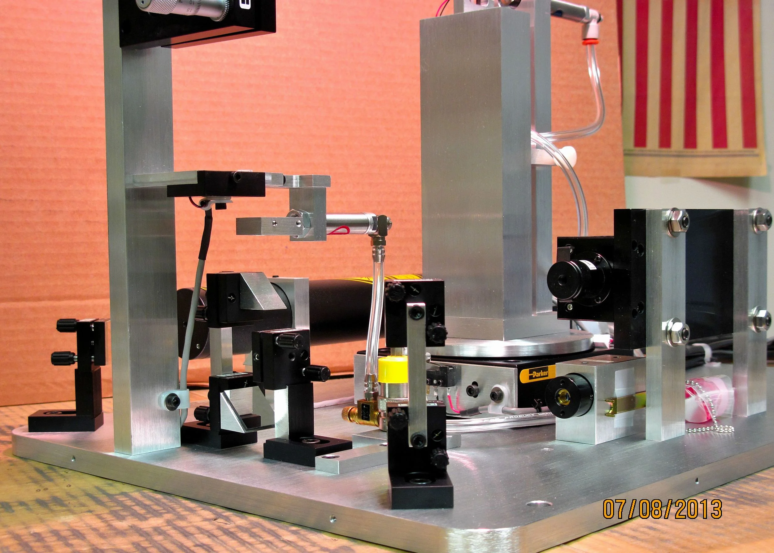
When light is coupled into an optical waveguide, light is scattered out of the surface of the guide as the light propagates down the guide.   Options 2010-WGL1 or 2010-WGL2 measure loss of planar optical waveguides by scanning a fiber optic probe and photodetector down the length of the propagating streak to measure the light intensity scattered from the surface of the guide (See Figs 1 and 2).  The assumption is that at every point on the propagating streak the light scattered from the surface and picked up by the fiber is proportional to the light which remains within the guide.  The best exponential fit to the resulting intensity vs distance curve yields the loss in db/cm.  This method offers the advantages of quickness (typical measurement time, including the exponential fit, is 2-3 minutes) and simplicity (absolutely no sample preparation beyond creation of the layers which form the guide is required).

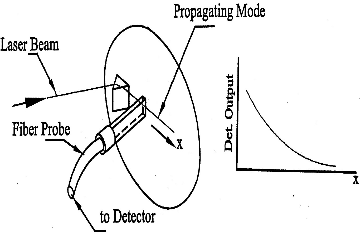
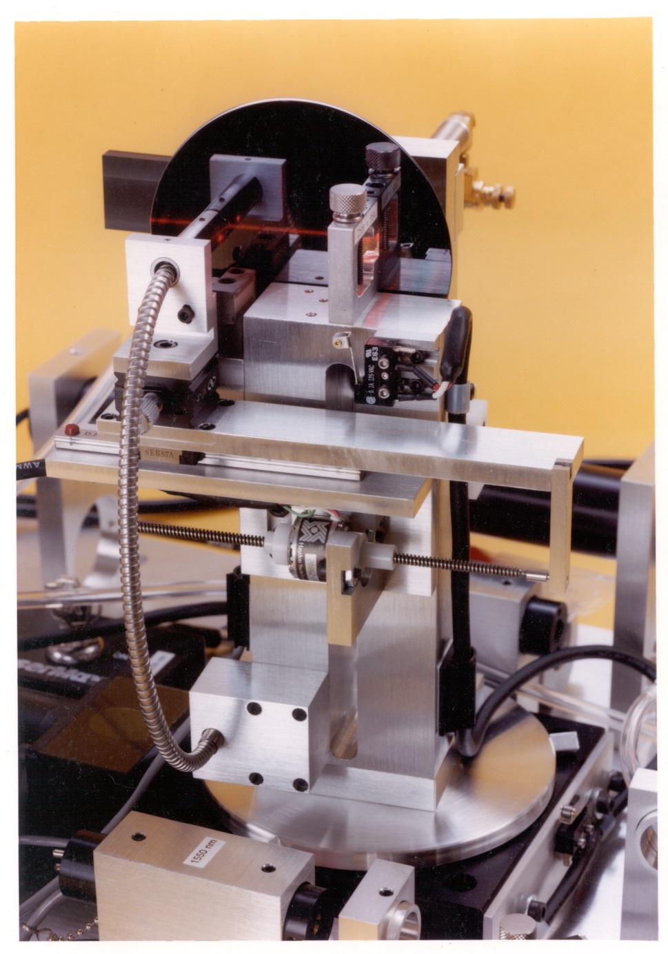
          Fig 1.  Schematic of loss measurement option                              Fig 2.  Loss measurement hardware            

Comparison to other methods:  The optical fiber method is identical in concept to the CCD camera approach for measuring the decay of the propagating streak but the camera must have very uniform response sensitivity over the full array.  With the scanning fiber method, only a small single-element silicon or InGaAs detector is used and spatial uniformity is not an issue.  In addition, for loss measurements beyond 1100 nm a high quality (and very expensive) spatially uniform IR camera is not required. 

Various two and three-prism coupling approaches have also been used to provide accurate loss results. In the typical two prism technique, one prism is used to couple light into the guide and another prism is moved down the guide to couple out and measure the light remaining within the guide at multiple points.  With this technique it is, however, very difficult to ensure that the coupling efficiency into the guide at the first prism is not changed as the second movable prism is brought into and out of contact with the sample.  Unless the coupling faces of the prisms lie precisely in the same planes and the samples themselves are extremely flat, mechanical stresses as the second prism is clamped to the sample can cause a change in the coupling efficiency or possibly complete loss of contact at the first prism.  To overcome this problem, various three prism approaches have been proposed to compensate for coupling efficiency changes at the first prism.  The main problem with these approaches is that the apparatus is mechanically quite complex and measurements are slow because of the need to couple and decouple the sample to the movable prism multiple times while monitoring that the coupling efficiency of the first prism does not change.

Another technique involves using a single prism to couple light into a sample and then immersing the sample into a bath filled with index matching fluid to couple out the light remaining within the guide.  This technique is limited to relatively low index guides (n ~ 1.7 or less) since the index of the fluid must be closely matched to the index of the guide and the maximum index available for matching fluids is limited.  Higher index fluids, moreover, are costly and often caustic or even poisonous, and use of a variety of different fluids may be required if working with waveguides over a range of indices.  In addition, waveguide materials, especially polymers, may react either obviously or more subtly when placed in contact with the matching fluids, leading to changes in loss behavior.  A final requirement is that the sample must usually be cut or broken into a long narrow piece because of bath size/shape limitations.  Cutting or breaking samples invariably generates large numbers of particles which can settle onto the sample surface and, unless extreme care is taken, it is difficult to avoid some scratching of the sample surface.   While normal measurements of index and thickness are relatively tolerant of surface scratches or small particles, surface scattering losses, which often dominate the loss behavior, are extremely sensitive to the introduction of particles and scratches.

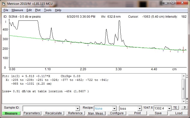
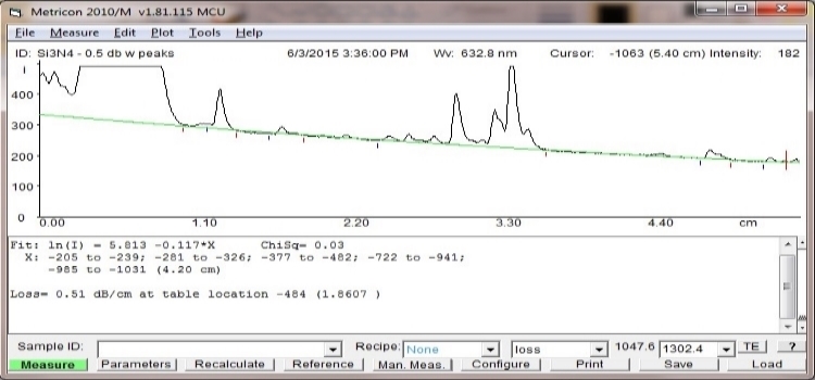
The scanning fiber method offers the advantages of mechanical and operational simplicity, speed, elimination of costly or toxic index matching fluids, and absolutely no sample preparation, but samples must exhibit some surface scattering loss to provide a means of sampling the light intensity within the guide.   In our experience, this is rarely a significant limitation since even low loss waveguides (below a few tenths of a db/cm) usually provide more than enough scattered light to be measurable.  A more important requirement, is that the scattering behavior of the sample surface be uniform for the propagation path over which loss is measured.  If, for example, one part of the streak scatters more than another, the scattered light at each point is not an accurate representation of the light remaining within the guide and the resulting intensity vs distance curve may not shown an exponential shape.   While the 2010/M system displays the optimum fitted exponential superimposed on the raw intensity vs distance curve (see sample measurements below), and it is easy for the user to recognize if the pattern deviates from exponential behavior, accuracy of the loss measurement is reduced when samples exhibit non-exponential patterns.  However, since surface scattering is an important mechanism of waveguide loss (and often the dominant mechanism) if scattering efficiency changes spatially over the surface of the sample, this really means that the loss itself (however it is measured) is changing spatially over the surface of the sample and there is no one single loss figure which is representative of the entire sample.   So the presence of a non-exponential curve is an important piece of information in itself, alerting the user that the loss of the sample may be spatially dependent. 
 
Loss measurement range:  The 2010/M's loss measurement option can be used  over the range from ~20 db/cm to ~ 0.1 db/cm (see sample measurements below).  Minimum loss measurable depends on how much light is scattered from the guide and whether the loss profile exhibits significant non-exponential behavior due to spatial variation in the surface scattering efficiency (see discussion above).  The best method of ensuring that the loss measurement option provides good characterization for a particular class of guides is to submit samples to Metricon for evaluation.
 
Waveguide index range measurable:  1.0 to 3.35 (with appropriate prism).  

Repeatability:  For guides which exhibit essentially exponential behavior, measurements taken at various points on the sample are usually repeatable to ±5% or ±0.05 db/cm, whichever is greater.  For guides with significantly non-exponential decay, measurement of individual propagation paths are usually repeatable to ±5% or less (i.e., a 1 db/cm measurement will vary by ±0.05 db/cm) but results may vary by ±20% depending on the exact path which the streak traces down the sample and point defects (scratches, particles) encountered in the path of the propagating beam.

Accuracy:  The science of loss measurement is in its infancy and no standards are available which permit certification of absolute loss accuracy.  However, observance of an essentially exponential loss decay profile is good evidence that the sample is conforming to theory and the loss measurement apparatus is measuring the decay profile accurately.  In the absence of a universally accepted loss accuracy standards, we invite and encourage comparative measurements between our apparatus and other techniques.

Wavelength measuring range:  From 400 to 1064 nm with silicon detector (option 2010-WGL1) or 600 to 1600 nm with InGaAs detector (option 2010-WGL2).

Sample size:  While measurements can often be made for  propagation distances of 25-30 mm from the coupling point, propagation distances of 40-50 mm are desirable, especially for low loss guides.  Any sample shape can be accommodated (circular, square, long and narrow).  The length of the profiling scan is user adjustable with a maximum scan length of 55 mm.  The fiber position is driven by a linear stepper motor with a linear resolution of 20 steps/mm, resulting in typical intensity patterns of 200 to 1000 data points.

Measurement procedure:  The rotary table is first positioned so that the desired mode is excited and a propagating streak is obtained (this is easily done even if the beam is invisible).  The fiber is then driven by a stepper motor into close proximity to the prism (at the start of the streak).  The fiber is then automatically scanned down the propagation path and the intensity vs distance profile is displayed on the computer monitor.  With a mouse, the user then selects the parts of the pattern to be used in the loss calculation, avoiding obvious peaks caused by scratches, particles, or other surface imperfections.  Loss in db/cm is then calculated automatically by a least squares fit to the intensity data and the resulting exponential fit is superimposed over the intensity profile.  To improve the fit, the portion of the intensity pattern included in the calculation can then be refined or changed and the loss recalculated. At any point, loss intensity patterns and results can be saved to disk or printed out on the system printer.  The entire process, from locating the mode to the final loss calculation, requires approximately 3-5 minutes.